In this case study we will use the Sales, Customer and Stores tables of the Mondrian Database in conjunction with a variety of processors and generate the output into different file formats. The data manipulations we will illustrate are extraction, merging, filtering, derivation, caching and transformation.
Before we begin, you should ensure the Mondrian datasource is configured as described in the section called “Using the JDBC/ODBC bridge driver”.
Adding the DataSources
Launch Elixir Repertoire. Choose or create a new file system or folder for this case study and from the popup menu choose Add->Datasource. In the DataSource Wizard that appears select the JDBC DataSource. Click the Next button.
In the Define JDBC DataSource screen enter the DataSource name as Store. Select the JDBC/ODBC bridge(Sun JVM) as the driver specification. Enter the URL as jdbc:odbc:MondrianFoodMart. Click the Next button.
In the SQL window add the following query:
Select * from Store
Click the Next button and then click the Infer Schema button. Similarly, add the Sales data source with SQL:
Select * from Sales_Fact_1997
Again, infer the schema. Similarly, add a Customer data source. In the SQL window enter:
Select * from Customer
and again infer the schema.
Add a Composite DataSource named Case Study.
Creating a Composite DataSource
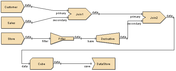
After adding the Composite DataSource, it will open automatically. We are going to create the diagram as shown in Figure 4.70, “Case Study Composite Diagram”. Select the Customer DataSource drag and place it on the diagram. Repeat the process for the Sales DataSource and then the Store DataSource.
Add the additional processors and connections as shown in Figure 4.70, “Case Study Composite Diagram”. In your version you will notice the link from Cube to DataStore is dashed because the tool cannot identify the schema for this flow until the cache has a schema inferred. With the diagram created, we can walk through the flow and set the various processor properties.
Join 1
In the Options tab window enter If no matching secondary: Discard record. If multiple matching secondary: Repeat primary for every secondary.
Change to the secondary tab and select the customer_id field in the "primary" column against the customer_id field of the secondary data source.
This configuration corresponds to an inner join, so records from the primary are only retained if a matching secondary record exists. In this case, only customers that have made purchases (have sales records) will be retained.
Filter
In the Filter#1 select Equals from the When condition column corresponding to the store_country field. Enter condition as USA.
The output from this part of the flow will only contain records where the store_country field has the value USA.
Derivative
Select the Derived tab and click the Add Column button to invoke the Add Column dialog box.
Enter name as grocery_meat_sum. Select Data Type as Integer. Enter value as given below:
grocery+meat
On clicking the Ok button the column is added to the wizard.
We've defined a new column grocery_meat_sum which contains the sum of grocery and meat fields.
Join 2
In the Options tab window enter If no matching secondary: Discard record and If multiple matching secondary: Repeat primary for each secondary.
Choose the Secondary tab and select the store_id field in the "primary" column against the store_id field of the secondary data source and click the Finish button.
Again we have used an inner join so records are only fetched based on a match with the secondary input. Because the secondary input filters out all countries except USA, the Join will discard all non-US customer sales from the primary datasource.
Cube
In the Cube Hierarchies screen click the Add button.
The Add Hierarchy dialog box pops up. Enter name as Location. Select store_country from the Schema column and click the > button. So the store_country is added to the Hierarchy Elements list. Similarly add the store_state and store_city to the Hierarchy Elements list. This creates a three-level hierarchy.
On clicking the Ok button the hierarchy column is added to the Wizard. Click the Next button.
On the Cube Axes screen, select gender and click > button to add the field to the Column Dimensions list box. Select Location and click > button to add the field to the Row Dimensions list box. Click the Next button.
On the Cube Measures screen, click the Add button. The Add Measure dialog box pops up. Select store_sales and the function Sum, leave the Pattern blank. Clicking Ok to add the measure to the Cube.
Similarly, add a measure for Average(store_sales) then Click the Next button.
The next screen allows cube options to be configured. We will leave the options at their default values, so click next again and infer the schema. This operation may take a while as it is analyzing hundreds of thousands of records. If you have previously executed the flow then the cache will have already been created and the inference will be faster.
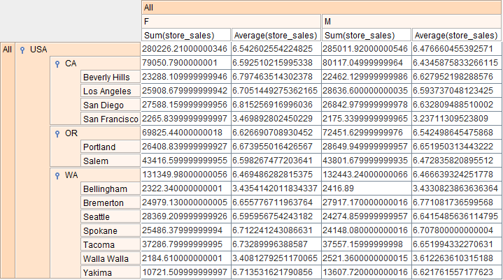
You should notice that after we've inferred the schema that the flow connector from the Cube to the DataStore has changed from a dashed line to a solid line, indicating that a schema is now defined for this link. We can test the process so far by selecting the Cube processor and choosing View Cube from the popup menu. The output is displayed as shown in Figure 4.71, “View Cube Output”.
The sum and average of sales for the male and female customers for the different cities belonging to specific States of USA are displayed.
DataStore
You can choose a few different kinds of output for the records we have processed, for this walkthrough we have chosen XML, MySQL and Oracle.
XML: Invoke the DataStore Wizard and set the following properties:
Select XML file from the Type combo box. Click the Next button.
Enter the URL as file:/C:/Output.xml (choose an appropriate location for your operating system) and click the Finish button.
Select the DataStore, and select Generate from the popup menu. The XML file will be generated and saved in the specified location.
MySQL: Before generating the MySQL JDBC DataStore, the MySQL driver file must be copied to the Elixir Repertoire ext folder. The tool must be launched once the jar is in place, as the jar is only loaded at startup. (Note if using Elixir Repertoire Remote, then the ext folder is on the server.)
Invoke the DataStore Wizard and set the following properties:
Select JDBC from the Type combo box. Click the Next button.
Select MySQL in the suggestions combo box.
On selecting the Driver Suggestion, the Driver class name and the URL are automatically displayed in the corresponding text boxes.
The URL is entered as jdbc:mysql://localhost:3306/test. Where test is the dbname, localhost can be replaced by the IP address of MySQL server if it isn't running on the same machine and 3306 is the port number.
Enter DataOutput as the table name.
Select the DataStore and choose Generate from the popup menu. The MySQL JDBC DataStore is generated and saved in the specified location.
Oracle: Before generating the Oracle JDBC DataStore, the Oracle driver file must be copied to the ext folder (on the client for the Designer, or on the server for the Remote). This ensures the Oracle driver is loaded into the class path when the tool is launched.
Invoke the DataStore Wizard and set the following properties:
Select JDBC from the Type combo box. Click the Next button.
Select Oracle in the suggestions combo box.
On selecting the Driver Suggestion, the Driver class name and the URL are automatically displayed in the corresponding text boxes.
The URL as jdbc:oracle:thin:@localhost:1521:ELX. Where localhost should be replaced by the IP address of the Oracle server if it isn't running on the same machine. The number 1521 is the port number and ELX is the database name.
Enter DataOutput as the table name.
Select the DataStore and choose Generate from the popup menu. The Oracle JDBC DataStore is generated and saved in the specific location.

